Long-read single-cell tutorial

This tutorial shows a simple workflow for pre-processing long-read single-cell RNA-seq using our tools flexiplex and nailpolish. We will take you through:

1. Extracting 10x barcodes from long-read single-cell data using flexiplex
2. Using flexiplex-filter to find the knee-point and shortlist barcodes
3. Demultiplexing reads with flexiplex
4. Cleaning reads and deduplicating UMIs with nailpolish
5. Aligning to a reference using minimap2
6. Quantification with oarfish (single-cell mode) to get a count matrix
7. Loading counts in R/Seurat and plotting a UMAP

A basic understanding of RNA sequencing data analysis is assumed. Prior experience with single-cell data will be helpful, as discussion of concepts such as UMIs, knee plots and empty drops will not be discussed here. The pipeline presented here is not an endorsement or recommendation for the best combination of software, as there are many option of tools at each step. These tools were primarily chosen for their usability (particularly for beginners). Questions and feedback (positive or negative) is very welcome on the tutorial and should be posted on our issue page, or by emailing the authors of flexiplex.

---

0. Prerequisites

Before beginning, the following packages must be installed or already available on a linux based system:

• flexiplex and flexiplex-filter
• nailpolish
• minimap2
• oarfish
• R and seurat

You will also need to download the demo dataset, scmixology2_250k.fastq.gz

wget --content-disposition https://ndownloader.figshare.com/files/57350216

This file is a subset of the scMixology replicate 2 data generated and published by Tan et al., Genome Biology, 2021 and rebase called by You et al., Genome Biology, 2023. It contains single cell sequencing data from a mixture of five lung cancer cell-lines (HCC827, H1975, H838, A549 and H2228) generated using 10x 3’ version 3 and Oxford Nanopore Technologies. We have subset down to just 250 thousand reads from the 250 most variable genes, to make the tutorial run in a reasonable time frame.

You will also need to download the human reference transcriptome, for the quantification step:

wget https://ftp.ebi.ac.uk/pub/databases/gencode/Gencode_human/release_48/gencode.v48.transcripts.fa.gz
gunzip gencode.v48.transcripts.fa.gz

1. Barcode discovery

To begin the data analysis, we will first need to find out which single-cell barcodes are present in the dataset. This can be done by running flexiplex in discovery mode (with the barcode list parameter, -k, missing):

gunzip -c scmixology2_250k.fastq.gz | flexiplex -d 10x3v3 -f 0 > 1_flexiplex.out

The output should look something like:

FLEXIPLEX 1.02.5
Using predefined settings for 10x3v3.
Adding flank sequence to search for: CTACACGACGCTCTTCCGATCT
Setting barcode to search for: ????????????????
Setting UMI to search for: ????????????
Adding flank sequence to search for: TTTTTTTTT
Setting max flanking sequence edit distance to 8
Setting max barcode edit distance to 2
Setting max flanking sequence edit distance to 0
For usage information type: flexiplex -h
No filename given... getting reads from stdin...
Searching for barcodes...
0.01 million reads processed..
0.02 million reads processed..
0.03 million reads processed..
0.04 million reads processed..
0.05 million reads processed..
0.06 million reads processed..
0.07 million reads processed..
0.08 million reads processed..
0.09 million reads processed..
0.1 million reads processed..
0.2 million reads processed..
Number of reads processed: 250000
Number of reads where a barcode was found: 112261
Number of reads where more than one barcode was found: 1422
All done!

You’ll see that the number of reads where a barcode was found is less than half, but this is okay because we have intentionally selected just the best quality read (-f 0 means no sequencing errors in the flank around the barcode). You’ll also see that there are some reads were multiple barcodes are found, so called chimeric reads. Flexiplex will chop these reads to make two (or more), when it’s running in demultiplexing mode later. We typically find 2-15% of reads being chimeric in this type of data. If you see a much larger fraction in your own dataset (>20%) you may have a data quality issues that needs addressing.

The key output from this step is a file called “flexiplex_barcodes_counts.txt” which lists the number of reads for each barcode, and will be used for generating a knee plot in the next step.

CTCCGATCATGGCCAC	1090
CATCGCTCAAGTAGTA	1050
GGGACCTTCTTGATTC	1025
TCATTTGTCACGGTCG	1009
GGAGGATTCTTCTAAC	946
AATCACGGTCCTCCTA	943
ATAGACCCACCGTCTT	923
AGCGCCACAATCCAGT	907
GCCCAGACAACACAAA	881
ATGCCTCGTCAAGCCC	867
...

2. Barcode filtering

Now, we are ready to refine the barcode list to a short list of high-quality barcodes. This is commonly done using a ‘knee plot’. A knee plot visualises the counts (reads or UMIs) per barcode by plotting the number of counts (y-axis) against barcode rank, after ranking on the number of counts (x-axis). For good-quality data, we tend to see a sudden drop in this distribution, giving the shape of a knee. Barcodes below the inflection point tend to have much lower counts and correspond to dead or dying cells, empty drops, or false barcodes, and should be removed. flexiplex-filter is a Python script packaged with flexiplex that will automatically identify the inflection point of the knee plot, reporting only the barcodes ranked above it, and (optionally) removing barcodes not present in a known list—such as the inclusion list provided by Cell Ranger. Check the flexiplex documentation carefully to make sure you have correctly installed flexiplex-filter, as it requires an extra step beyond the installation of flexiplex.

To run:

flexiplex-filter flexiplex_barcodes_counts.txt > flexiplex_barcodes_final.txt

Optionally, if you have an inclusion list from Cell Ranger (but this is not required):

flexiplex-filter -w [inclusion_list] flexiplex_barcodes_counts.txt > flexiplex_barcodes_final.txt

It’s always a good idea to manually check that flexiplex-filter has chosen the correct inflection point. This can be done by generating an interactive plot of the barcode frequencies (needs to done on a system with GUI support):

flexiplex-filter -g flexiplex_barcodes_counts.txt

In this case, is appears to have chosen well.

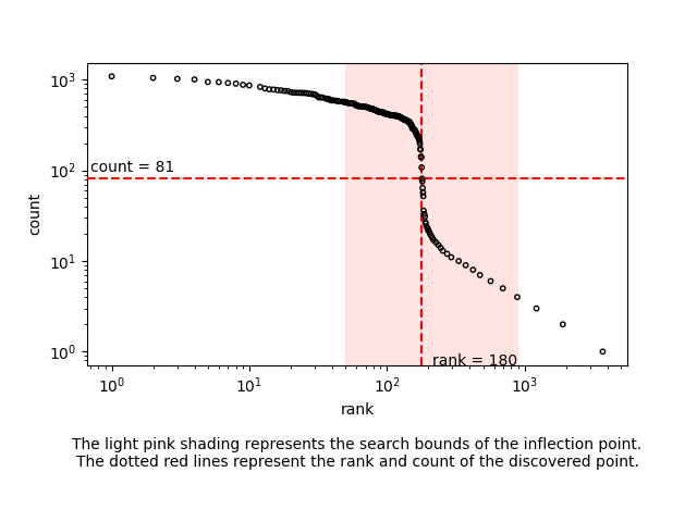
In our example, flexiplex-filter picked the 180 most frequent barcodes, which is close to the number of cells expected in this dataset. The process above will also work for samples with many more cells, and has been tested on datasets with tens of thousands of cells.

3. Barcode demultiplexing

Now we have a short-list of barcodes. We will run flexiplex a second time to actually assign each read to one of these barcodes, trim off the 10x primer/adapter sequence, and chop any chimeric reads:

gunzip -c scmixology2_250k.fastq.gz | flexiplex -d 10x3v3 -k flexiplex_barcodes_final.txt > scmixology2_250k.demultiplexed.fastq

The output of this look like:

FLEXIPLEX 1.02.5
Using predefined settings for 10x3v3.
Adding flank sequence to search for: CTACACGACGCTCTTCCGATCT
Setting barcode to search for: ????????????????
Setting UMI to search for: ????????????
Adding flank sequence to search for: TTTTTTTTT
Setting max flanking sequence edit distance to 8
Setting max barcode edit distance to 2
Setting known barcodes from flexiplex_barcodes_final.txt
Number of known barcodes: 180
For usage information type: flexiplex -h
No filename given... getting reads from stdin...
File flexiplex_reads_barcodes.txt already exists, overwriting.
Searching for barcodes...
0.01 million reads processed..
0.02 million reads processed..
0.03 million reads processed..
0.04 million reads processed..
0.05 million reads processed..
0.06 million reads processed..
0.07 million reads processed..
0.08 million reads processed..
0.09 million reads processed..
0.1 million reads processed..
0.2 million reads processed..
Number of reads processed: 250000
Number of reads where a barcode was found: 213458
Number of reads where more than one barcode was found: 5923
All done!

And you see that we are able to find barcodes in 85% of reads, with a 2.7% chimeric rate - both of these metrics are great. The read ID now contains the barcode (CB) and UMI (UB) information needed for downstream analysis:

head -n2 scmixology2_250k.demultiplexed.fastq

@GCCCGAACAATACCCA_GCATAAATTGTA#82f7a317-c081-4d86-bbb3-60926dce0db9_+1of1	CB:Z:GCCCGAACAATACCCA	UB:Z:GCATAAATTGTA
TTTTTTTTTTTTTTGTATTTTTAGTAGAGACGGGGTTTCACCATATTGGCCAGGCTGGTCTCGAACTCCTGACCTCATCATCCACCTGCCTTAGCCTCCCAAAATGCTGGGATTACAGGCATGAGCCACCGCACCCGGCCAGGAATTGCTTCTTATGGATGAACAAAGAAAATAGTTTCCTGAGATGGTATCTACTCTGTGAAGATGCACAACATTGTTGAAATGACAACAAAGGATCTGAATATTACATAAACTTGTTGATAAAAACAGTGGCAGGGTTTGAGATCATTGATTCAGTTTTGAAAGAAGTTCTACTGTGGGTAAAAATGCCATCAAACAGCATCACATGCTGCAGAGAAATCTTTCATGAAAGGAAGAATCAATCGATATGTATCCTCCATTTTGTCTTATTTTAAAAATTTGCCACAGCCACTCCAACCTTCAGTAACTACTACCTTGATCTGTCAGCAGCCATCAACATCAAGGCAACAGACCCTCCCACCAGCAAAAAAATTACAACTTGCTGAAGGCTCAGATGATCATTACCATTTTTTAACAATATTTTAAGATAGGTGTGTACATTGTTTTTAGACATAATCTATTGCATACTTAATAGACTTCTACAGTAATAGTGCAAAACATAACCTTTATGTACACTAGGGAACCAAAAATTTACACGTGACTCCTTTTATTTTGATGGTCTGGAACTGAGTCCACAGTATCTCCAAGGTATGCCTATATTGACTGATGAATAAACAAAATGTGGTATAGCCATACAATGGAATATTGTTCAGTCACAAAAAGAATAACATTCTGATACATGCTACAACATAGATGAACCTTGAAAATATTATGCTAAGTGAAAGAAGTCAGACACAAAAGACAAGTATTATATGATTCCATTTATATAAAATGTCCAGGATAGTCAAATCAACGAGAGACCAAAAAGTAGATTAATGGTTGACAGAGGCTGAAGGTAGGGAGGAAATGGGGAGTGACTTTAATGGGTACAGGGTTTTAGATAAAAGAAAATGTTCTGGAATTAGTGGTGATGCACAACCTTGTACAACCTTTTTGCAATATAGTGCAATAAGACAATATTGTACAATCTTGTTTATATACTAAAGCCATTAAATTACACACTTTAAAGGGTGCATTTTATGACATGGGAAGTGTACATTAAAAATAAATAACCCCATGTACTCTGCGTTGATACCACTGCTTGGCCATTAGGCCTGTAAACAATACGTAACTTG

4. Deduplication and polishing

As single-cell data often contains multiple reads for each unique barcode and UMI combination, we need to deduplicate reads to a single barcode/UMI combination. This is often done after alignment and during quantification (ie. only counting a barcode and UMI combination once). However, nailpolish allows this deduplication to be performed earlier, and uses the duplicate reads to generate consensus sequences - hence improving the read accuracy whilst also deduplicating.

Nailpolish works in two steps. First the fastq file is indexed.

nailpolish index scmixology2_250k.demultiplexed.fastq

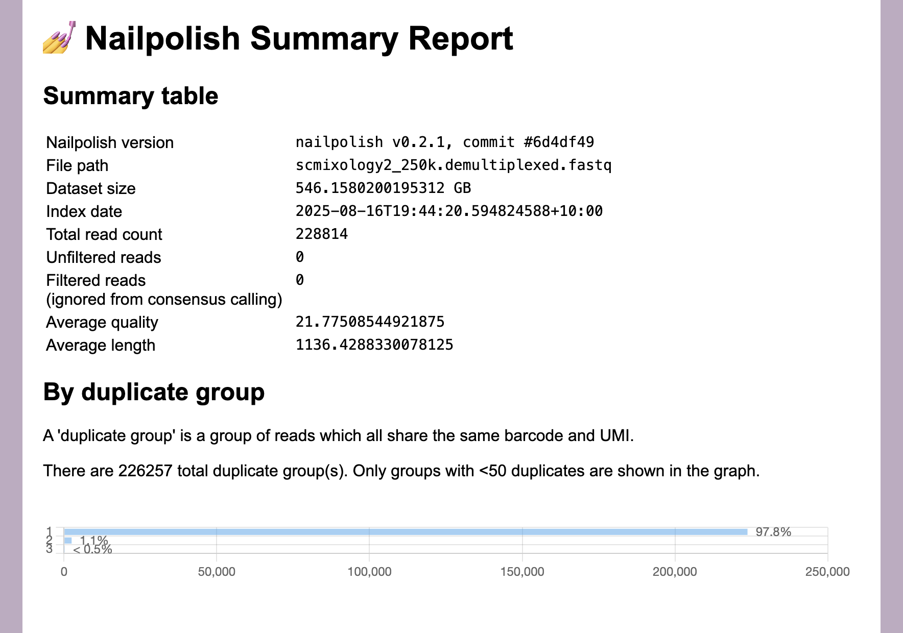
At this point you can use the output to examine the duplication rate within the data.

nailpolish summary scmixology2_250k.demultiplexed.fastq

Loading scmixology2_250k.demultiplexed.summary.html in a browser shows that the duplicate rate is low (around 2%). That’s because this tutorial uses a small subset the data, but a range of 5-40% would be typical for long-read single-cell data, and depends on saturation levels.

Now we can perform the consensus calling:

nailpolish consensus scmixology2_250k.demultiplexed.fastq > scmixology2_250k.demultiplexed.deduplicated.fastq

The resulting data will be a mixture of original (singlet) and consensus (duplicated) reads, which each have a unique barcode and UMI. The barcode and UMI are encoded in the CB and UB tags in the read ID line, as before.

5. Read Mapping

We are now ready to align the reads. As we’ll be using oarfish for quantification, mapping is done against the reference transcriptome. In this instance gencode (downloaded in step 0).

minimap2 --rev-only -y -ax map-ont gencode.v48.transcripts.fa \
      scmixology2_250k.demultiplexed.deduplicated.fastq |\
      samtools view -b |\
      samtools sort -t CB \
      -o scmixology2_250k.demultiplexed.deduplicated.bam

The “–rev-only” flag tells minimap2 to only map to the reverse strand. We do this because after demultiplexing, the reads are oriented in the anti-sense direction (note this might be different for protocols other than 10x 3’). Some chimeric reads will be present even after the demultiplexing and chopping, and this reduces their impact.

The “-y” flag here is important as it tell minimap2 to add the barcode and UMI (CB and UB) tags into the bam (these will be used by oarfish):

samtools view scmixology2_250k.demultiplexed.deduplicated.bam | head -n2
processed_16225_1	272	ENST00000457540.1|ENSG00000225630.1|OTTHUMG00000002336.1|OTTHUMT00000006718.1|MTND2P28-201|MTND2P28|1044|unprocessed_pseudogene|	1	0	1607S6M1D102M3D23M2D34M1D107M1D58M1I26M1D11M1D16M3D46M1I2M1I73M2D7M1I8M1D49M1I6M1D139M1D8M1I13M3D140M1D19M3D49M1I69M15S	*	0	0*	*	NM:i:56	ms:i:1735	AS:i:1726	nn:i:0	tp:A:S	cm:i:99	s1:i:682	de:f:0.0445	rl:i:230	MI:Z:AAAGAACAGCGATCGA_CCCGATTTGCGT	nI:i:16225	CB:Z:AAAGAACAGCGATCGA	UB:Z:CCCGATTTGCGT	nT:Z:simplex
processed_174462_1	272	ENST00000414273.1|ENSG00000237973.1|OTTHUMG00000002333.2|OTTHUMT00000006715.2|MTCO1P12-201|MTCO1P12|1543|unprocessed_pseudogene|	1082	0	1069S19M1I30M1I57M1I5M1D38M1I50M3I150M2D110M67S	*	0	0	*	*	NM:i:20	ms:i:813	AS:i:810	nn:i:0	tp:A:S	cm:i:52	s1:i:360	de:f:0.0365	rl:i:30	MI:Z:AAAGAACAGCGATCGA_TACCCTGAGTGT	nI:i:174462	CB:Z:AAAGAACAGCGATCGA	UB:Z:TACCCTGAGTGT	nT:Z:simplex

samtools view -b converts the output to bam format, and samtools sort -t CB, sorts the reads by cell barcode which is required by oarfish

6. Transcript Quantification

Next we quantify the transcript expression using oarfish.

oarfish --alignments scmixology2_250k.demultiplexed.deduplicated.bam \
        --single-cell \
        --filter-group no-filters \
        --model-coverage \
        -o scmixology2_250k

This generates the following three files which are needed for count data analysis:

scmixology2_250k.barcodes.txt
scmixology2_250k.count.mtx
scmixology2_250k.features.txt

7. Count analysis

At this point your count matrix can be analysed is whatever way makes the most sense for your experiment. Here we show a simple example using R and Seurat to generate a UMAP of the cells. This part of the tutorial is designed to be short, but for a real dataset there are several more QC and data exploration steps we would encourage you to perform. There are many excellent guides for single-cell analysis such as these: Seurat or introduction to single-cell analysis

The following will be done within R, so it’s assumed you already have that installed on your system. First we will load in the oarfish transcript count matrix and create a Seurat object from it:

library(Matrix)
library(Seurat)

stem <- "scmixology2_250k"
counts <- t(Matrix::readMM(paste0(stem, ".count.mtx")))
features <- read.delim(paste0(stem, ".features.txt"), header = FALSE, stringsAsFactors = FALSE)
barcodes <- readLines(paste0(stem, ".barcodes.txt"))

rownames(counts) <- features[[1]]
colnames(counts) <- barcodes
seu <- CreateSeuratObject(counts = counts)

Now we need to check the data quality. Specifically, checking if there are ‘poor’ quality cells that need to be filtered out. These tend to be dead/dying cells or empty drops. Most of these will have been removed already during our flexiplex-filter step above, but some may remain:

seu[["percent.mt"]] <- PercentageFeatureSet(seu, pattern = "-MT-")
FeatureScatter(seu, feature1 = "nCount_RNA", feature2 = "percent.mt") |
FeatureScatter(seu, feature1 = "nCount_RNA", feature2 = "nFeature_RNA")

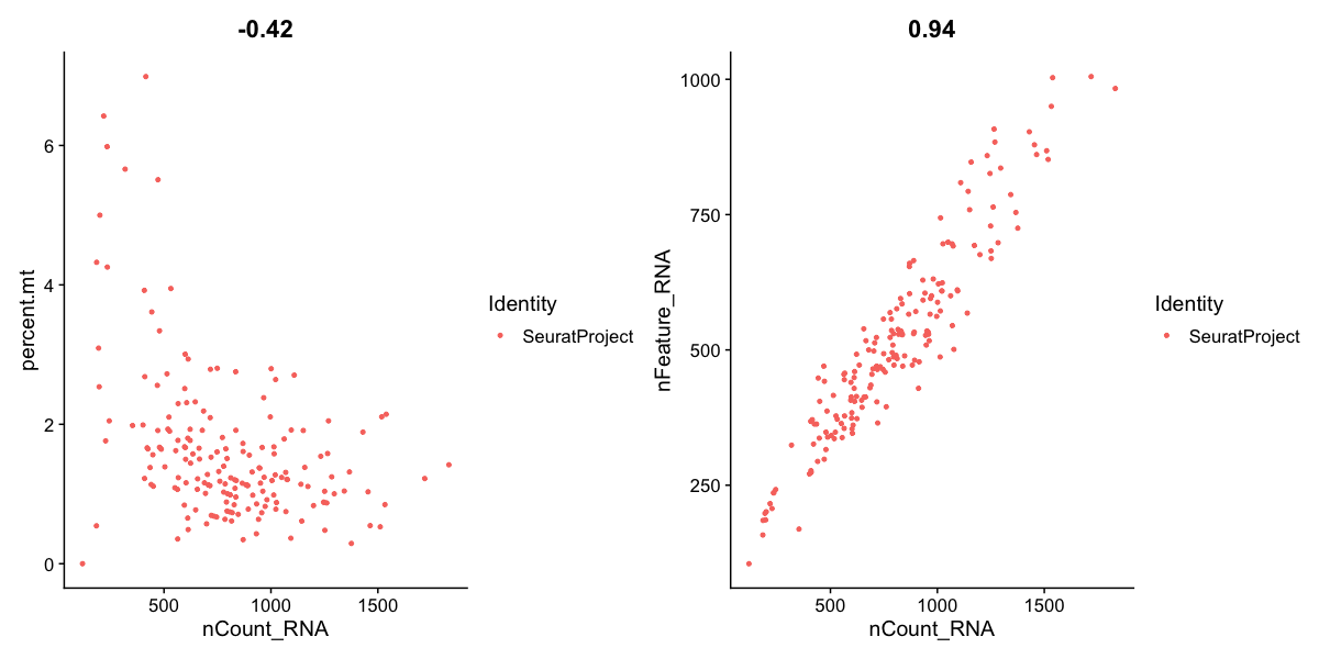
This step calculates the fraction of UMIs coming from mitochondrial genes - which tend to be higher for poor quality cells. As you will see here there is a sprinkling of cells above 4% with low count, that may be bad quality. The % you filter on will need to be adjusted for each dataset, and may be higher than this (e.g. 10-20% is still typical). We can also check the number of features (transcripts) with one or more UMI count and the number of total UMI counts, per cells. Again we see a group with low features and counts.

We will filter these out:

seu <- subset(seu, subset = nFeature_RNA > 250 & percent.mt < 4)

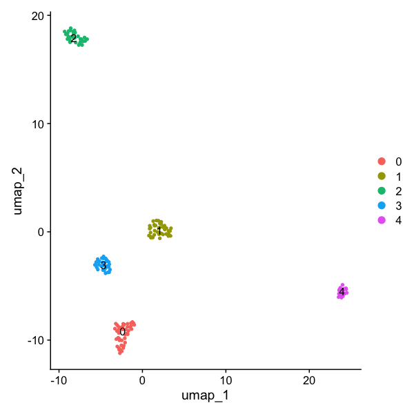
We are now ready to look at the cell clustering. If all has gone well, we would expect five distinct groups - corresponding to the five different cell-lines.

seu <- NormalizeData(seu)
seu <- FindVariableFeatures(seu, nfeatures = 500)
seu <- ScaleData(seu)
seu <- RunPCA(seu, npcs = 10)

seu <- FindNeighbors(seu, dims = 1:10)
seu <- FindClusters(seu, resolution = 0.6, random.seed = 2022)

seu <- RunUMAP(seu, dims = 1:10)

DimPlot(seu, reduction = "umap", label = TRUE)

As hoped, we get a UMAP showing five well defined clusters of cells:

The tutorial has been completed!

Further analyses you could consider undertaking with long-read single-cell data, are:

• Genotyping cells by known driver mutations with flexiplex - website, paper
• Calling fusion genes with JAFFAL - website, paper, tutorial
• Testing for differential transcript usage with Isopod - website

If you prefer an all-on-one pipeline for long-read single-cell pre-processing, take a look at FLAMES or Bambu-clump.

This tutorial was written by Nadia M. Davidson, and tested by Oliver Cheng and Shian Su from the Walter and Eliza Hall Institute, 2025. Questions, comments and feedback are most welcome.